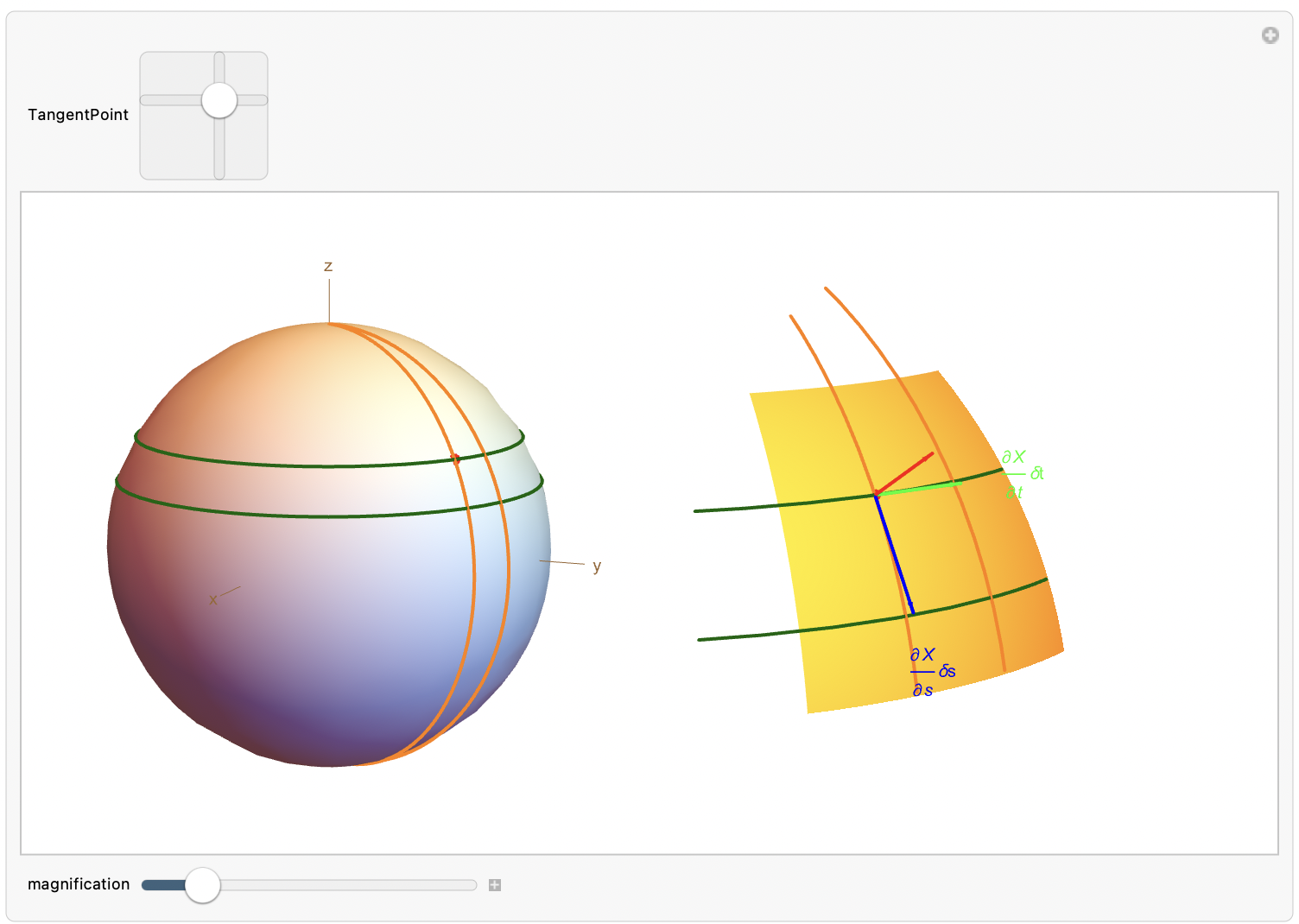
Local Linearity viewed in a Microscope:
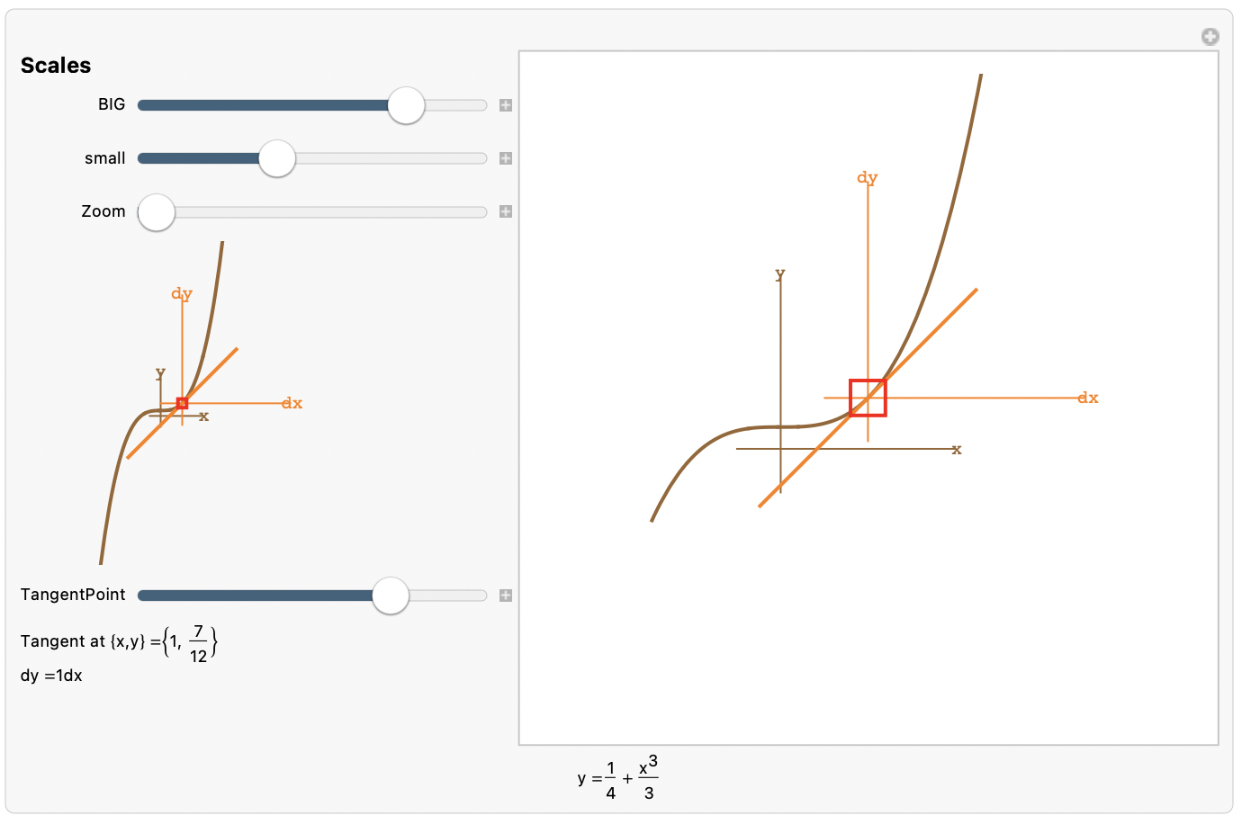
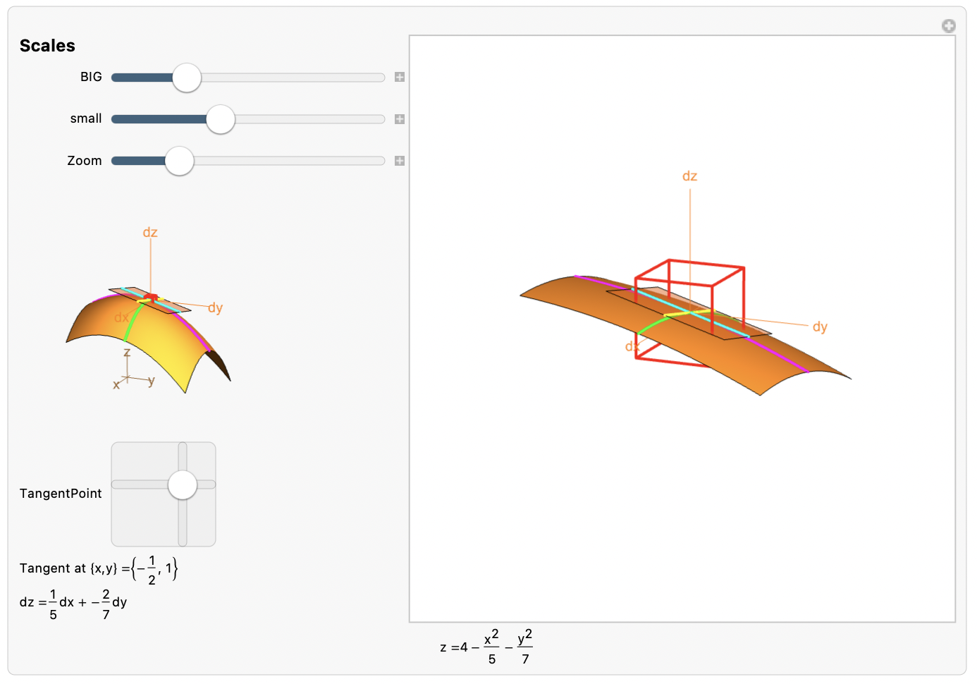
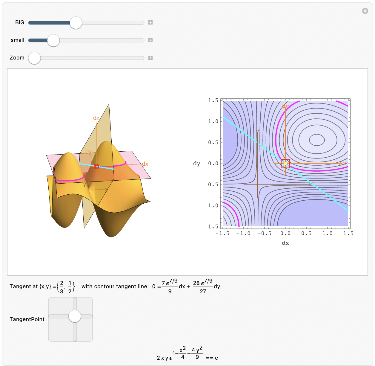
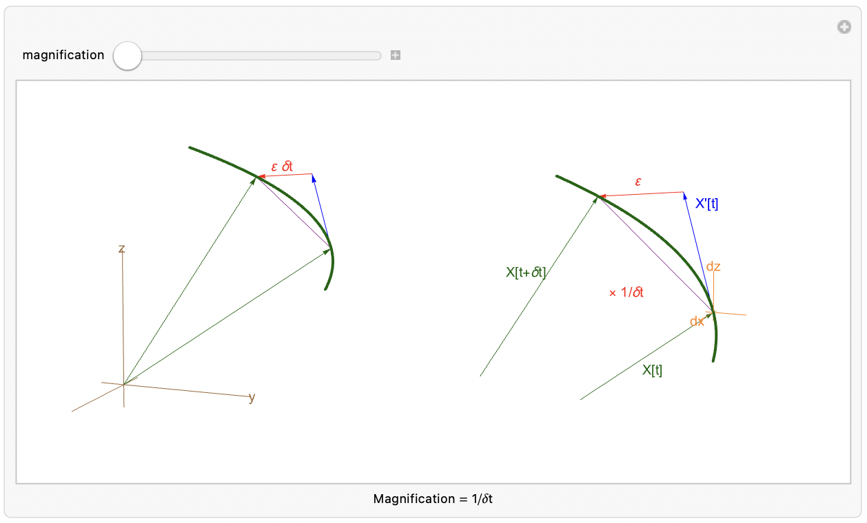
A geometric interpretation of the tangent computation procedure is that the result is what we would see in an infinitely (or “sufficiently”) powerful microscope. Advanced Calculus using Mathematica has interactive animations that allow users to magnify for the various tangents as well as view other important "linearizations" as follows:
Zooming in on an Explicit Curve
Zooming in on an Explicit Surface
Zooming in on a Parametric Curve
Zooming in on a Parametric Surface
Zooming in on an increment of a Flow
Microscopic Divergence and Swirl in 2D
Microscopic Divergence and Curl in 3D
Zooming in at an Equilibrium of a Flow
Analytical Local Linearity
The analytical explanation of zooming to the linear approximation in the case of an explicit curve or surface is based directly on the “small oh” formula:

Extra conditions for implicit and parametric graphs are explained in the text. Local linearity and “zooming” also applies to vector fields and flows as described in the novel topics below.
Local linearity & Integration
The idea of many integral formulas is to sum the “microscopic amounts” and show that micrsocopic errors don’t accumulate. (The idea that errors that are small in the microscope don’t accumulate is called Duhamel’s Principle.) An important basic case of this idea arises in the Fundamental Theorem of Calculus in 1 variable. That example shows how a uniform approximation of the derivative (smoothness or continuous differentiability) is the needed technical condition. Other examples of sums of microscopic amounts animated in the text are:
Arclength: Theorem 9.7.1
Work or Flux: 2D
Green’s Theorem: 2D
Surface Area: 3D
Stokes’ and Gauss’Theorems